04 - MSM analysis
In this notebook, we will cover how to analyze an MSM and how the modeled processes correspond to MSM spectral properties.
Maintainers: [@cwehmeyer](https://github.com/cwehmeyer), [@marscher](https://github.com/marscher), [@thempel](https://github.com/thempel), [@psolsson](https://github.com/psolsson)
Remember: - to run the currently highlighted cell, hold ⇧ Shift and press ⏎ Enter; - to get help for a specific function, place the cursor within the function’s brackets, hold ⇧ Shift, and press ⇥ Tab; - you can find the full documentation at PyEMMA.org.
%matplotlib inline
import matplotlib.pyplot as plt
import matplotlib as mpl
import numpy as np
import mdshare
import pyemma
Case 1: preprocessed, two-dimensional data (toy model)
We load the two-dimensional trajectory from an archive using numpy, directly discretize the full space using \(k\)-means clustering, visualize the marginal and joint distributions of both components as well as the cluster centers, and show the implied timescale (ITS) convergence:
file = mdshare.fetch('hmm-doublewell-2d-100k.npz', working_directory='data')
with np.load(file) as fh:
    data = fh['trajectory']

cluster = pyemma.coordinates.cluster_kmeans(data, k=50, max_iter=50)
its = pyemma.msm.its(
    cluster.dtrajs, lags=[1, 2, 3, 5, 7, 10], nits=3, errors='bayes')

fig, axes = plt.subplots(1, 3, figsize=(12, 3))
pyemma.plots.plot_feature_histograms(data, feature_labels=['$x$', '$y$'], ax=axes[0])
pyemma.plots.plot_density(*data.T, ax=axes[1], cbar=False, alpha=0.1)
axes[1].scatter(*cluster.clustercenters.T, s=15, c='C1')
axes[1].set_xlabel('$x$')
axes[1].set_ylabel('$y$')
axes[1].set_xlim(-4, 4)
axes[1].set_ylim(-4, 4)
axes[1].set_aspect('equal')
pyemma.plots.plot_implied_timescales(its, ylog=False, ax=axes[2])
fig.tight_layout()
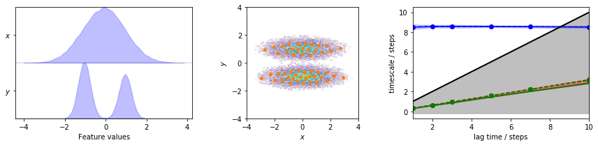
The plots show us the marginal (left panel) and joint distributions along with the cluster centers (middle panel). The implied timescales are converged (right panel).
Before we proceed, let’s have a look at the implied timescales error
bars. They were computed from a Bayesian MSM, as requested by the
errors='bayes' argument of the pyemma.msm.its() function. As
mentioned before, Bayesian MSMs incorporate a sample of transition
matrices. Target properties such as implied timescales can now simply be
computed from the individual matrices. Thereby, the posterior
distributions of these properties can be estimated. The ITS plot shows a
confidence interval that contains \(95\%\) of the Bayesian samples.
bayesian_msm = pyemma.msm.bayesian_markov_model(cluster.dtrajs, lag=1, conf=0.95)
For any PyEMMA method that derives target properties from MSMs, sample
mean and confidence intervals (as defined by the function argument
above) are directly accessible with sample_mean() and
sample_conf(). Further, sample_std() is available for computing
the standard deviation. In the more general case, it might be
interesting to extract the full sample of a function evaluation with
sample_f(). The syntax is equivalent for all those functions.
sample_mean = bayesian_msm.sample_mean('timescales', k=1)
sample_conf_l, sample_conf_r = bayesian_msm.sample_conf('timescales', k=1)

print('Mean of first ITS: {:f}'.format(sample_mean[0]))
print('Confidence interval: [{:f}, {:f}]'.format(sample_conf_l[0], sample_conf_r[0]))
Please note that sample mean and maximum likelihood estimates are not identical and generally do not provide numerically identical results.
Now, for the sake of simplicity we proceed with the analysis of a maximum likelihood MSM. We estimate it at lag time \(1\) step.
msm = pyemma.msm.estimate_markov_model(cluster.dtrajs, lag=1)
and check for disconnectivity. The MSM is constructed on the largest set
of discrete states that are (reversibly) connected. The
active_state_fraction and active_count_fraction show us the
fraction of discrete states and transition counts from our data which
are part of this largest set and, thus, used for the model:
print('fraction of states used = {:f}'.format(msm.active_state_fraction))
print('fraction of counts used = {:f}'.format(msm.active_count_fraction))
The fraction is, in both cases, \(1\) and, thus, we have no disconnected states (which we would have to exclude from our analysis).
If there were any disconnectivities in our data (fractions \(<1\)),
we could access the indices of the active states (members of the
largest connected set) via the active_set attribute:
print(msm.active_set)
With this potential issue out of the way, we can extract our first
(stationary/thermodynamic) property, the stationary_distribution or,
as a shortcut, pi:
print(msm.stationary_distribution)
print('sum of weights = {:f}'.format(msm.pi.sum()))
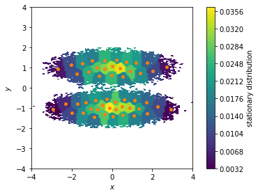
The attribute msm.pi tells us, for each discrete state, the absolute
probability of observing said state in global equilibrium.
Mathematically speaking, the stationary distribution \(\pi\) is the
left eigenvector of the transition matrix \(\mathbf{T}\) to the
eigenvalue \(1\):
We can use the stationary distribution to, e.g., visualize the weight of the dicrete states and, thus, to highlight which areas of our feature space are most probable. Here, we show all data points in a two dimensional scatter plot and color/weight them according to their discrete state membership:
fig, ax, misc = pyemma.plots.plot_contour(
    *data.T, msm.pi[cluster.dtrajs[0]],
    cbar_label='stationary distribution',
    method='nearest', mask=True)
ax.scatter(*cluster.clustercenters.T, s=15, c='C1')
ax.set_xlabel('$x$')
ax.set_ylabel('$y$')
ax.set_xlim(-4, 4)
ax.set_ylim(-4, 4)
ax.set_aspect('equal')
fig.tight_layout()
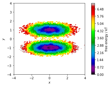
The stationary distribution can also be used to correct the
pyemma.plots.plot_free_energy() function. This might be necessary if
the data points are not sampled from global equilibrium.
In this case, we assign the weight of the corresponding discrete state
to each data point and pass this information to the plotting function
via its weights parameter:
fig, ax, misc = pyemma.plots.plot_free_energy(
    *data.T,
    weights=msm.pi[cluster.dtrajs[0]],
    legacy=False)
ax.set_xlabel('$x$')
ax.set_ylabel('$y$')
ax.set_xlim(-4, 4)
ax.set_ylim(-4, 4)
ax.set_aspect('equal')
fig.tight_layout()
We will see further uses of the stationary distribution later. But for now, we continue the analysis of our model by visualizing its (right) eigenvectors. First, we notice that the first right eigenvector is a constant \(1\).
eigvec = msm.eigenvectors_right()
print('first eigenvector is one: {} (min={}, max={})'.format(
    np.allclose(eigvec[:, 0], 1, atol=1e-15), eigvec[:, 0].min(), eigvec[:, 0].max()))
Second, the higher eigenvectors can be visualized as follows:
fig, axes = plt.subplots(1, 3, figsize=(12, 3))
for i, ax in enumerate(axes.flat):
    pyemma.plots.plot_contour(
        *data.T, eigvec[cluster.dtrajs[0], i + 1], ax=ax, cmap='PiYG',
        cbar_label='{}. right eigenvector'.format(i + 2), mask=True)
    ax.scatter(*cluster.clustercenters.T, s=15, c='C1')
    ax.set_xlabel('$x$')
    ax.set_xlim(-4, 4)
    ax.set_ylim(-4, 4)
    ax.set_aspect('equal')
axes[0].set_ylabel('$y$')
fig.tight_layout()
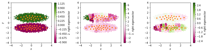
The right eigenvectors can be used to visualize the processes governed by the corresponding implied timescales. The first right eigenvector (always) is \((1,\dots,1)^\top\) for an MSM transition matrix and it corresponds to the stationary process (infinite implied timescale).
The second right eigenvector corresponds to the slowest process; its entries are negative for one group of discrete states and positive for the other group. This tells us that the slowest process happens between these two groups and that the process relaxes on the slowest ITS (\(\approx 8.5\) steps).
The third and fourth eigenvectors show a larger spread of values and no clear grouping. In combination with the ITS convergence plot, we can safely assume that these eigenvectors contain just noise and do not indicate any resolved processes.
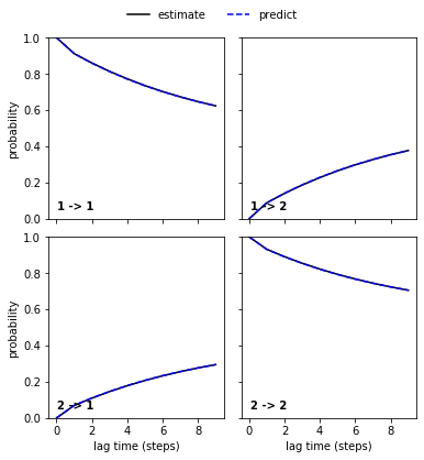
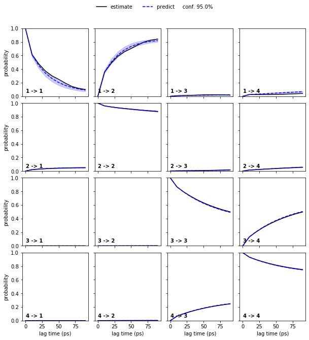
We then continue to validate our MSM with a CK test for \(2\) metastable states which are already indicated by the second right eigenvector.
nstates = 2
pyemma.plots.plot_cktest(msm.cktest(nstates));
We now save the model to do more analyses with PCCA++ and TPT in the follow-up notebook:
cluster.save('nb4.pyemma', model_name='doublewell_cluster', overwrite=True)
msm.save('nb4.pyemma', model_name='doublewell_msm', overwrite=True)
bayesian_msm.save('nb4.pyemma', model_name='doublewell_bayesian_msm', overwrite=True)
Case 2: low-dimensional molecular dynamics data (alanine dipeptide)
We fetch the alanine dipeptide data set, load the backbone torsions into memory, directly discretize the full space using \(k\)-means clustering, visualize the margial and joint distributions of both components as well as the cluster centers, and show the ITS convergence to help selecting a suitable lag time:
pdb = mdshare.fetch('alanine-dipeptide-nowater.pdb', working_directory='data')
files = mdshare.fetch('alanine-dipeptide-*-250ns-nowater.xtc', working_directory='data')

feat = pyemma.coordinates.featurizer(pdb)
feat.add_backbone_torsions(periodic=False)
data = pyemma.coordinates.load(files, features=feat)
data_concatenated = np.concatenate(data)

cluster = pyemma.coordinates.cluster_kmeans(data, k=100, max_iter=50, stride=10)
dtrajs_concatenated = np.concatenate(cluster.dtrajs)

its = pyemma.msm.its(
    cluster.dtrajs, lags=[1, 2, 5, 10, 20, 50], nits=4, errors='bayes')

fig, axes = plt.subplots(1, 3, figsize=(12, 3))
pyemma.plots.plot_feature_histograms(
    np.concatenate(data), feature_labels=['$\Phi$', '$\Psi$'], ax=axes[0])
pyemma.plots.plot_density(*data_concatenated.T, ax=axes[1], cbar=False, alpha=0.1)
axes[1].scatter(*cluster.clustercenters.T, s=15, c='C1')
axes[1].set_xlabel('$\Phi$')
axes[1].set_ylabel('$\Psi$')
pyemma.plots.plot_implied_timescales(its, ax=axes[2], units='ps')
fig.tight_layout()
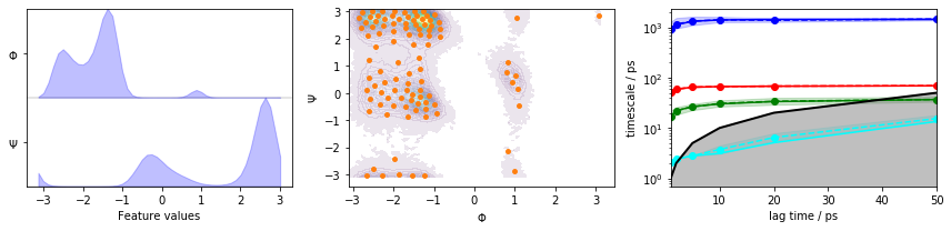
The plots show us the marginal (left panel) and joint distributions along with the cluster centers (middle panel). The implied timescales are converged (right panel).
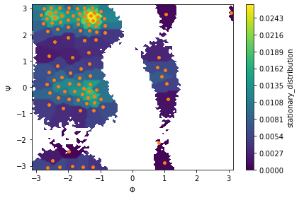
We then estimate an MSM at lag time \(10\) ps and visualize the stationary distribution by coloring all data points according to the stationary weight of the discrete state they belong to:
msm = pyemma.msm.estimate_markov_model(cluster.dtrajs, lag=10, dt_traj='1 ps')

print('fraction of states used = {:f}'.format(msm.active_state_fraction))
print('fraction of counts used = {:f}'.format(msm.active_count_fraction))

fig, ax, misc = pyemma.plots.plot_contour(
    *data_concatenated.T, msm.pi[dtrajs_concatenated],
    cbar_label='stationary_distribution',
    method='nearest', mask=True)
ax.scatter(*cluster.clustercenters.T, s=15, c='C1')
ax.set_xlabel('$\Phi$')
ax.set_ylabel('$\Psi$')
fig.tight_layout()
Next, we visualize the first six right eigenvectors:
eigvec = msm.eigenvectors_right()
print('first eigenvector is one: {} (min={}, max={})'.format(
    np.allclose(eigvec[:, 0], 1, atol=1e-15), eigvec[:, 0].min(), eigvec[:, 0].max()))

fig, axes = plt.subplots(2, 3, figsize=(12, 6))
for i, ax in enumerate(axes.flat):
    pyemma.plots.plot_contour(
        *data_concatenated.T, eigvec[dtrajs_concatenated, i + 1], ax=ax, cmap='PiYG',
        cbar_label='{}. right eigenvector'.format(i + 2), mask=True)
    ax.scatter(*cluster.clustercenters.T, s=15, c='C1')
    ax.set_xlabel('$\Phi$')
    ax.set_ylabel('$\Psi$')
fig.tight_layout()
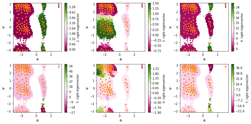
Again, we have the \((1,\dots,1)^\top\) first right eigenvector of the stationary process.
The second to fourth right eigenvectors illustrate the three slowest processes.
Eigenvectors five, six, and seven indicate further processes which, however, relax faster than the lag time and cannot be resolved clearly.
We now proceed our validation process using a Bayesian MSM with four metastable states:
nstates = 4
bayesian_msm = pyemma.msm.bayesian_markov_model(cluster.dtrajs, lag=10, dt_traj='1 ps')
pyemma.plots.plot_cktest(bayesian_msm.cktest(nstates), units='ps');
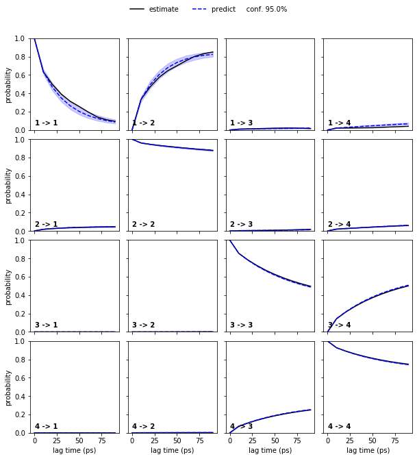
We note that four metastable states are a reasonable choice for our MSM.
In general, the number of metastable states is a modeler’s choice; it is adjusted to map the kinetics to be modeled. In the current example, increasing the resolution with a higher number of metastable states or resolving only the slowest process between \(2\) states would be possible. However, the number of states is not arbitrary as the observed processes in metastable state space need not be Markovian in general. A failed Chapman-Kolmogorov test can thus also hint to a bad choice of the metastable state number.
In order to perform further analysis, we save the model to disk:
cluster.save('nb4.pyemma', model_name='ala2_cluster', overwrite=True)
msm.save('nb4.pyemma', model_name='ala2_msm', overwrite=True)
bayesian_msm.save('nb4.pyemma', model_name='ala2_bayesian_msm', overwrite=True)
Exercise 1
Load the heavy atom distances into memory, TICA (lag=3 and
dim=2), discretize with 100 \(k\)-means centers and a stride of
\(10\), and show the ITS convergence.
Solution
feat = pyemma.coordinates.featurizer(pdb)
pairs = feat.pairs(feat.select_Heavy())
feat.add_distances(pairs, periodic=False)
data = pyemma.coordinates.load(files, features=feat)
tica = pyemma.coordinates.tica(data, lag=3, dim=2)
tica_concatenated = np.concatenate(tica.get_output())
cluster = pyemma.coordinates.cluster_kmeans(tica, k=100, max_iter=50, stride=10)
dtrajs_concatenated = np.concatenate(cluster.dtrajs)
its = pyemma.msm.its(
cluster.dtrajs, lags=[1, 2, 5, 10, 20, 50], nits=4, errors='bayes')
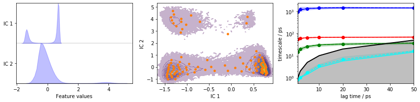
fig, axes = plt.subplots(1, 3, figsize=(12, 3))
pyemma.plots.plot_feature_histograms(tica_concatenated, feature_labels=['IC 1', 'IC 2'], ax=axes[0])
pyemma.plots.plot_density(*tica_concatenated.T, ax=axes[1], cbar=False, alpha=0.3)
axes[1].scatter(*cluster.clustercenters.T, s=15, c='C1')
axes[1].set_xlabel('IC 1')
axes[1].set_ylabel('IC 2')
pyemma.plots.plot_implied_timescales(its, ax=axes[2], units='ps')
fig.tight_layout()
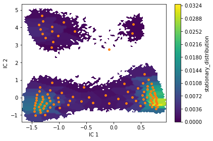
Exercise 2
Estimate an MSM at lag time \(10\) ps with dt_traj='1 ps' and
visualize the stationary distribution using a two-dimensional colored
scatter plot of all data points in TICA space.
Solution
msm = pyemma.msm.estimate_markov_model(cluster.dtrajs, lag=10, dt_traj='1 ps')

print('fraction of states used = {:f}'.format(msm.active_state_fraction))
print('fraction of counts used = {:f}'.format(msm.active_count_fraction))

fig, ax, misc = pyemma.plots.plot_contour(
    *tica_concatenated.T, msm.pi[dtrajs_concatenated],
    cbar_label='stationary_distribution',
    method='nearest', mask=True)
ax.scatter(*cluster.clustercenters.T, s=15, c='C1')
ax.set_xlabel('IC 1')
ax.set_ylabel('IC 2')
fig.tight_layout()
Exercise 3
Visualize the first six right eigenvectors.
Solution
eigvec = msm.eigenvectors_right()
print('first eigenvector is one: {} (min={}, max={})'.format(
    np.allclose(eigvec[:, 0], 1, atol=1e-15), eigvec[:, 0].min(), eigvec[:, 0].max()))

fig, axes = plt.subplots(2, 3, figsize=(12, 6))
for i, ax in enumerate(axes.flat):
    pyemma.plots.plot_contour(
        *tica_concatenated.T, eigvec[dtrajs_concatenated, i + 1], ax=ax, cmap='PiYG',
        cbar_label='{}. right eigenvector'.format(i + 2), mask=True)
    ax.scatter(*cluster.clustercenters.T, s=15, c='C1')
    ax.set_xlabel('IC 1')
    ax.set_ylabel('IC 2')
fig.tight_layout()
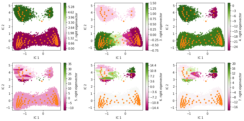
Can you already guess from eigenvectors two to four which the metastable states are?
Exercise 4
Estimate a Bayesian MSM at lag time \(10\) ps and perform/show a CK test for four metastable states.
Solution
bayesian_msm = pyemma.msm.bayesian_markov_model(cluster.dtrajs, lag=10, dt_traj='1 ps')

nstates = 4
pyemma.plots.plot_cktest(bayesian_msm.cktest(nstates), units='ps');
Exercise 5
Save the MSM, Bayesian MSM and Cluster objects to the same file as
before. Use the model names ala2tica_msm, ala2tica_bayesian_msm
and ala2tica_cluster, respectively. Further, include the TICA object
with model name ala2tica_tica.
Solution
cluster.save('nb4.pyemma', model_name='ala2tica_cluster', overwrite=True)
msm.save('nb4.pyemma', model_name='ala2tica_msm', overwrite=True)
bayesian_msm.save('nb4.pyemma', model_name='ala2tica_bayesian_msm', overwrite=True)
tica.save('nb4.pyemma', model_name='ala2tica_tica', overwrite=True)
Wrapping up
In this notebook, we have learned how to analyze an MSM and how to
extract kinetic information from the model. In detail, we have used -
the active_state_fraction, active_count_fraction, and
active_set attributes of an MSM object to see how much (and which
parts) of our data form the largest connected set represented by the
MSM, - the stationary_distribution (or pi) attribute of an MSM
object to access its stationary vector, - the eigenvectors_right()
method of an MSM object to access its (right) eigenvectors,
For visualizing MSMs or kinetic networks we used -
pyemma.plots.plot_density() - pyemma.plots.plot_contour() and -
pyemma.plots.plot_cktest().